The use of the count function has always been a topic of debate, especially in MySQL. As PostgreSQL gains popularity, does it have similar issues? Let’s explore the behavior of the count function in PostgreSQL through practical experiments.
Building a Test Database
Create a test database and a test table. The test table includes three fields: an auto-increment ID, a creation time, and content. The auto-increment ID field is the primary key.
create database performance_test;

create table test_tbl (id serial primary key, created_at timestamp, content varchar(512));
Generating Test Data
Use the generate_series function to generate auto-increment IDs, the now() function for the created_at column, and repeat(md5(random()::text), 10) to generate 10 strings of 32-character md5 hashes for the content column. Use the following statement to insert 10 million records for testing.
performance_test=# insert into test_tbl select generate_series(1,10000000),now(),repeat(md5(random()::text),10);
INSERT 0 10000000
Time: 212184.223 ms (03:32.184)
Thoughts Triggered by the count Statement
By default, PostgreSQL does not display SQL execution time, so it needs to be enabled manually for comparison in subsequent tests.
\timing on
The performance difference between count(*) and count(1) is a frequently discussed issue. Let’s execute a query using both count(*) and count(1).
performance_test=# select count(*) from test_tbl;
  count
----------
 10000000
(1 row)

Time: 115090.380 ms (01:55.090)

performance_test=# select count(1) from test_tbl;
  count
----------
 10000000
(1 row)

Time: 738.502 ms
The speed difference between the two queries is significant. Does count(1) really offer such a performance boost? Let’s run the queries again.
performance_test=# select count(*) from test_tbl;
  count
----------
 10000000
(1 row)

Time: 657.831 ms

performance_test=# select count(1) from test_tbl;
  count
----------
 10000000
(1 row)

Time: 682.157 ms
The first query is very slow, but the subsequent three are much faster and similar in time. This raises two questions:
- Why is the first query so slow?
- Is there really a performance difference between count(*) and count(1)?
Query Caching
Use the explain statement to re-execute the query.
explain (analyze,buffers,verbose) select count(*) from test_tbl;
The output is as follows:
 Finalize Aggregate  (cost=529273.69..529273.70 rows=1 width=8) (actual time=882.569..882.570 rows=1 loops=1)
   Output: count(*)
   Buffers: shared hit=96 read=476095
   ->  Gather  (cost=529273.48..529273.69 rows=2 width=8) (actual time=882.492..884.170 rows=3 loops=1)
         Output: (PARTIAL count(*))
         Workers Planned: 2
         Workers Launched: 2
         Buffers: shared hit=96 read=476095
         ->  Partial Aggregate  (cost=528273.48..528273.49 rows=1 width=8) (actual time=881.014..881.014 rows=1 loops=3)
               Output: PARTIAL count(*)
               Buffers: shared hit=96 read=476095
               Worker 0: actual time=880.319..880.319 rows=1 loops=1
                 Buffers: shared hit=34 read=158206
               Worker 1: actual time=880.369..880.369 rows=1 loops=1
                 Buffers: shared hit=29 read=156424
               ->  Parallel Seq Scan on public.test_tbl  (cost=0.00..517856.98 rows=4166598 width=0) (actual time=0.029..662.165 rows=3333333 loops=3)
                     Buffers: shared hit=96 read=476095
                     Worker 0: actual time=0.026..661.807 rows=3323029 loops=1
                       Buffers: shared hit=34 read=158206
                     Worker 1: actual time=0.030..660.197 rows=3285513 loops=1
                       Buffers: shared hit=29 read=156424
 Planning time: 0.043 ms
 Execution time: 884.207 ms
Note the shared hit, indicating that the data was cached in memory, explaining why subsequent queries are much faster than the first. Next, clear the cache and restart PostgreSQL.
service postgresql stop
echo 1 > /proc/sys/vm/drop_caches
service postgresql start
Re-execute the SQL statement, and it is much slower.
 Finalize Aggregate  (cost=529273.69..529273.70 rows=1 width=8) (actual time=50604.564..50604.564 rows=1 loops=1)
   Output: count(*)
   Buffers: shared read=476191
   ->  Gather  (cost=529273.48..529273.69 rows=2 width=8) (actual time=50604.508..50606.141 rows=3 loops=1)
         Output: (PARTIAL count(*))
         Workers Planned: 2
         Workers Launched: 2
         Buffers: shared read=476191
         ->  Partial Aggregate  (cost=528273.48..528273.49 rows=1 width=8) (actual time=50591.550..50591.551 rows=1 loops=3)
               Output: PARTIAL count(*)
               Buffers: shared read=476191
               Worker 0: actual time=50585.182..50585.182 rows=1 loops=1
                 Buffers: shared read=158122
               Worker 1: actual time=50585.181..50585.181 rows=1 loops=1
                 Buffers: shared read=161123
               ->  Parallel Seq Scan on public.test_tbl  (cost=0.00..517856.98 rows=4166598 width=0) (actual time=92.491..50369.691 rows=3333333 loops=3)
                     Buffers: shared read=476191
                     Worker 0: actual time=122.170..50362.271 rows=3320562 loops=1
                       Buffers: shared read=158122
                     Worker 1: actual time=14.020..50359.733 rows=3383583 loops=1
                       Buffers: shared read=161123
 Planning time: 11.537 ms
 Execution time: 50606.215 ms
shared read indicates that the cache was not hit. From this observation, we can infer that in the four queries from the previous section, the first query did not hit the cache, while the remaining three did.
Differences Between count(1) and count(*)
Next, let’s explore the differences between count(1) and count(*). Considering the initial four queries, the first used count(*), and the second used count(1), yet it still hit the cache. Doesn’t this indicate that count(1) and count(*) are the same?
In fact, PostgreSQL’s official response to the question “is there a difference performance-wise between select count(1) and select count(*)?” confirms this:
Nope. In fact, the latter is converted to the former during parsing.[2]
Since count(1) does not offer better performance than count(*), using count(*) is the better choice.
Sequence Scan and Index Scan
Next, let’s test the speed of count(*) with different data sizes. Write the query statement in a count.sql file and use pgbench for testing.
pgbench -c 5 -t 20 performance_test -r -f count.sql
Test the count statement execution time for data sizes ranging from 2 million to 10 million.
| Data Size | Count Time (ms) |
|---|---|
| 2 million | 738.758 |
| 3 million | 1035.846 |
| 4 million | 1426.183 |
| 5 million | 1799.866 |
| 6 million | 2117.247 |
| 7 million | 2514.691 |
| 8 million | 2526.441 |
| 9 million | 2568.240 |
| 10 million | 2650.434 |
Plot the time curve.
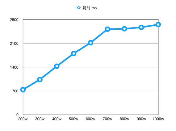
The trend of the curve changes between 6 million and 7 million data points. From 2 million to 6 million, it grows linearly, but after 6 million, the count time remains almost the same. Use the explain statement to check the execution of the count statement for 6 million and 7 million data points.
7 million:
 Finalize Aggregate  (cost=502185.93..502185.94 rows=1 width=8) (actual time=894.361..894.361 rows=1 loops=1)
   Output: count(*)
   Buffers: shared hit=16344 read=352463
   ->  Gather  (cost=502185.72..502185.93 rows=2 width=8) (actual time=894.232..899.763 rows=3 loops=1)
         Output: (PARTIAL count(*))
         Workers Planned: 2
         Workers Launched: 2
         Buffers: shared hit=16344 read=352463
         ->  Partial Aggregate  (cost=501185.72..501185.73 rows=1 width=8) (actual time=889.371..889.371 rows=1 loops=3)
               Output: PARTIAL count(*)
               Buffers: shared hit=16344 read=352463
               Worker 0: actual time=887.112..887.112 rows=1 loops=1
                 Buffers: shared hit=5459 read=118070
               Worker 1: actual time=887.120..887.120 rows=1 loops=1
                 Buffers: shared hit=5601 read=117051
               ->  Parallel Index Only Scan using test_tbl_pkey on public.test_tbl  (cost=0.43..493863.32 rows=2928960 width=0) (actual time=0.112..736.376 rows=2333333 loops=3)
                     Index Cond: (test_tbl.id < 7000000)
                     Heap Fetches: 2328492
                     Buffers: shared hit=16344 read=352463
                     Worker 0: actual time=0.107..737.180 rows=2344479 loops=1
                       Buffers: shared hit=5459 read=118070
                     Worker 1: actual time=0.133..737.960 rows=2327028 loops=1
                       Buffers: shared hit=5601 read=117051
 Planning time: 0.165 ms
 Execution time: 899.857 ms
6 million:
 Finalize Aggregate  (cost=429990.94..429990.95 rows=1 width=8) (actual time=765.575..765.575 rows=1 loops=1)
   Output: count(*)
   Buffers: shared hit=13999 read=302112
   ->  Gather  (cost=429990.72..429990.93 rows=2 width=8) (actual time=765.557..770.889 rows=3 loops=1)
         Output: (PARTIAL count(*))
         Workers Planned: 2
         Workers Launched: 2
         Buffers: shared hit=13999 read=302112
         ->  Partial Aggregate  (cost=428990.72..428990.73 rows=1 width=8) (actual time=763.821..763.821 rows=1 loops=3)
               Output: PARTIAL count(*)
               Buffers: shared hit=13999 read=302112
               Worker 0: actual time=762.742..762.742 rows=1 loops=1
                 Buffers: shared hit=4638 read=98875
               Worker 1: actual time=763.308..763.308 rows=1 loops=1
                 Buffers: shared hit=4696 read=101570
               ->  Parallel Index Only Scan using test_tbl_pkey on public.test_tbl  (cost=0.43..422723.16 rows=2507026 width=0) (actual time=0.053..632.199 rows=2000000 loops=3)
                     Index Cond: (test_tbl.id < 6000000)
                     Heap Fetches: 2018490
                     Buffers: shared hit=13999 read=302112
                     Worker 0: actual time=0.059..633.156 rows=1964483 loops=1
                       Buffers: shared hit=4638 read=98875
                     Worker 1: actual time=0.038..634.271 rows=2017026 loops=1
                       Buffers: shared hit=4696 read=101570
 Planning time: 0.055 ms
 Execution time: 770.921 ms
From these observations, it seems that PostgreSQL uses index scans for count operations when the data size is below a certain proportion of the table length. The official wiki also describes this:
It is important to realise that the planner is concerned with minimising the total cost of the query. With databases, the cost of I/O typically dominates. For that reason, “count(*) without any predicate” queries will only use an index-only scan if the index is significantly smaller than its table. This typically only happens when the table’s row width is much wider than some indexes’.[3]
According to a Stackoverflow response, count queries switch from index scans to full table scans when the count exceeds 3/4 of the table size.[4]
Conclusion
- Do not use count(1) or count(column name) instead of count(*).
- Count operations are inherently time-consuming.
- Count operations may use index scans or sequence scans, depending on the proportion of the count relative to the table size.
References
[1] In-depth Understanding of Cache in Postgres
[2] Re: performance difference in count(1) vs. count(*)?